Approximation Theory and Method part 2
Approximation operators
在前面的讨论中,我们得到了 best approximation 的一些性质. 但是实际上我们并不总是能有 best approximation 这么好的结果。那么我们能不能退而求其次,研究一下更具一般性的 approximation operators 呢?
We note that the operator $\boldsymbol X$ is defined to be a projection if the equation \(\boldsymbol{X}[\boldsymbol{X}(f)]=\boldsymbol{X}(f), \quad f \in \mathscr{B},\) is satisfied. Hence a sufficient condition for $X$ to be a projection is the equation \(X(a)=a, \quad a \in \mathscr{A}\) Most of the approximation methods that are considered in this book do satisfy condition (3.2), but an important exception is the Bernstein operator, which is discussed in Chapter 6. Sometimes $X(f)$ is written as $X f$.
The idea of a linear operator is also well known; namely, we define $X$ to be linear if the equation \(X(\lambda f)=\lambda \boldsymbol{X}(f)\)
holds for all $f \in \mathscr{B}$, where $\lambda$ is any real number, and if the equation \(\boldsymbol{X}(f+g)=\boldsymbol{X}(f)+\boldsymbol{X}(g)\) is obtained for all $f \in \mathscr{B}$ and for all $g \in \mathscr{B}$.
最好还是定义一下这些 approximation operator 的 norm.
Also we make frequent use of the norm of an approximation operator. The norm of $X$ is written as $\lVert X \rVert$, and it is the smallest real number such that the inequality \(\lVert \boldsymbol{X}(f) \rVert \leqslant\lVert \boldsymbol{X} \rVert\lVert f \rVert\) 或者可以这样写 \(\lVert \boldsymbol{X} \rVert = \sup _{ \lVert f \rVert \neq 0} \frac{\lVert \boldsymbol{X}(f) \rVert }{\lVert f \rVert}\) 这和我们定义矩阵时是类似的. 比如矩阵$A$ 的 norm: \(\lVert A \rVert = \sup _{ \lVert x \rVert \neq 0} \frac{\lVert Ax \rVert }{\lVert x \rVert}\) 关于 norm of approximation operator 的取值问题,可以考虑一个例子.
An example of an approximation operator that is useful because it is easy to apply is as follows. Let $\mathscr{B}$ be the space $\mathscr{C}[0,1]$ of real-valued functions that are continuous on $[0,1]$, and let $\mathscr{A}$ be the linear space $\mathscr{P}_1$ of all real polynomials of degree at most one. Then, in order that the calculation of an approximation to a function $f$ in $\mathscr{R}$ depends on only two function evaluations, we let $p$ be the polynomial in $\mathscr{A}$ that satisfies the interpolation conditions \(\left.\begin{array}{l} p(0)=f(0) \\ p(1)=f(1) \end{array}\right\rbrace\) Thus $p=X(f)$, where $X$ is a linear projection operator from $\mathscr{B}$ to $\mathscr{A}$. In order to define the norm of this operator we choose a norm for the space $\mathscr{C}[0,1]$. However, if the 2-norm \(\lVert f \rVert_2=\left\lbrace\int_0^1[f(x)]^2 \mathrm{~d} x\right\rbrace^{\frac{1}{2}}, \quad f \in \mathscr{C}[0,1],\) is used, we find that the operator $X$ is unbounded, because it is possible for $\lVert X f \rVert_2$ to be one when $\lVert f \rVert_2$ is arbitrarily small. It is therefore necessary to prefer the $\infty$-norm \(\lVert f \rVert_{\infty}=\max _{0 \leqslant x \leqslant 1}\lvert f(x) \rvert, \quad f \in \mathscr{C}[0,1]\) when considering approximation operators that are defined by interpolation conditions. In this case, because $p$ is in $\mathscr{P}_1$, equation (3.6) implies the inequality \(\begin{aligned} \lVert X(f) \rVert & =\lVert p \rVert \\ & =\max [\lvert p(0) \rvert,\lvert p(1) \rvert] \\ & =\max [\lvert f(0) \rvert,\lvert f(1) \rvert] \\ & \leqslant\lVert f \rVert, \quad f \in \mathscr{C}[0,1] . \end{aligned}\) 在这个例子中,我们的 approximation operator 可以理解为把 0 和 1 处,也就是函数的两端进行连线. 可以发现此时 2-norm 可以去到很大,而 inf-norm 是有上确界的.
Lebesgue constants
Theorem 3.1 Let $\mathscr{A}$ be a finite-dimensional linear subspace of a normed linear space $\mathscr{B}$, and let $X$ be a linear operator from $\mathscr{B}$ to $\mathscr{A}$ that satisfies the projection condition (3.2). For any $f$ in $\mathscr{B}$, let $d^*$ be the least distance \(d^*=\min _{a \in \mathbb{A}}\lVert f-a \rVert\) from $f$ to an element of $\mathscr{A}$. Then the error of the approximation $X(f)$ satisfies the bound \(\lVert f-X(f) \rVert \leqslant[1+\lVert X \rVert] d^*\) 在上面我们退而求其次,使用一个满足 projection 和 linearity 的 approximation operator 来进行逼近. 感觉这个逼近的结果和最优点有一段距离,在这里定理3.1 给出了一个上界: 肯定在最优附近的$[1+\lVert X \rVert]$范围内.
Polynomial approximations to differentiable functions
在后面我们会证明,对于任意一个函数$f \in \mathscr{C}[a, b]$,我们可以用多项式$p$进行逼近,并且可以让误差要多小有多小. \(\lVert f-p \rVert_{\infty} \leqslant \varepsilon\) 看起来这是一个很强,而且不错的结果.
Polynomial interpolation
所谓多项式插值,就是对多项式进行一个值的插()
比如有 $(n + 1)$ 组观测到的数据: $(x_i, y_i)$ for $i = 0,1,…,n$, 实际上背后的函数是$f$, 这个函数是什么函数都可以. 比如城市气温的函数, 我们想用多项式$p$进行逼近. 按照经验来看,比如我们有两个观测点,那我们能唯一确定一个 $p \in \mathscr P_1$, 如果有5个观测点,那用那我们能唯一确定一个 $p \in \mathscr P_4$.
关于$\mathscr P_n$, 我们知道$n$是多项式的最高次数. 比如 $p = 1+x$ 那么 $p \in \mathscr P _1$, $p = 1$ 那么 $p \in \mathscr P_0$
那多项式 $p = 0$ 是几次多项式呢?
可以考虑 $p = 0$ 的性质. 假设 $p \in \mathscr P_?$ 假设有个 $q \in \mathscr P_{4}$, $pq = 0$ 所以 $pq \in \mathscr P_{?}$.
所以感觉 $? = - \infty$ 蛮不错. 那就定义成 $p \in \mathscr P_{-\infty}$ .
希望在观测的地方,多项式的值就是实际函数的值. 那么这实际上就是一个解方程的问题: \(\left\lbrace\begin{array}{c} \sum c_i x_0^i=y_0 \\ \sum c_i x_1^i=y_1 \\ \vdots \\ \sum c_i x_n^i=y_n \end{array}\right.\) 想要知道这个方程组解的数量,实际上就是想知道 $\det(V)$, where $V$ is the Vandermonde matrix \(V=V\left(x_0, x_1, \cdots, x_m\right)=\left[\begin{array}{ccccc} 1 & x_0 & x_0^2 & \ldots & x_0^n \\ 1 & x_1 & x_1^2 & \ldots & x_1^n \\ 1 & x_2 & x_2^2 & \ldots & x_2^n \\ \vdots & \vdots & \vdots & \ddots & \vdots \\ 1 & x_m & x_m^2 & \ldots & x_m^n \end{array}\right]\) The determinant of a square Vandermonde matrix is called a Vandermonde polynomial or Vandermonde determinant. Its value is the polynomial \(\operatorname{det}(V)=\prod_{0 \leq i<j \leq n}\left(x_j-x_i\right)\) 我们的假设是每个观测的点都不一样,所以 $\operatorname{det}(V) \neq 0$. 也就是有唯一解.
在引入 Lagrange interpolation 之前,其实这个思想和中国剩余定理很相似. 不妨先复习复习中国剩余定理.
有物不知其数,三三数之剩二,五五数之剩三,七七数之剩二。问物几何?
也就是求解同余方程组: \(\left\lbrace\begin{aligned} x & \equiv 2 \quad\left(\bmod 3\right) \\ x & \equiv 3 \quad\left(\bmod 5\right) \\ x & \equiv 2 \quad \left(\bmod 7\right) \end{aligned}\right.\) 我们想知道,解的
- existence
- uniqueness
- how to find
首先确定解的范围. 可以注意到,如果 $n_1$ 是一个解,那么 $n_2 = n_1 + 105$ 也是一个可行解. 那么只考虑 $R = [1, 105]$ 中的可行解就行了.
如果 $n_1,n_2 \in R$ 是两个不同的解, 那么$n_1 - n_2$ 一定被 3, 5, 7 整除,但是注意到 $-104 \leq n_1 - n_2 \leq 104$,这样的 $n_1,n_2$ 并不存在. 所以,如果有在 $R$ 中的解,这个解是唯一的.
关于存在性, 考虑问题集: \(\left\lbrace\begin{aligned} x & \equiv 0,1,2 \quad\left(\bmod 3\right) \\ x & \equiv 0,1,2,3,4 \quad\left(\bmod 5\right) \\ x & \equiv 0,1,2,3,4,5,6 \quad \left(\bmod 7\right) \end{aligned}\right.\) 意思是,在 $\mod{}$ 后面的数字确定的情况下,一共有$3\times 5 \times 7 = 105$ 个可能的问题. 可能的解有 $\lvert R \rvert = 105$ 个, 每个问题的解都是唯一的, 不同问题的解肯定不一样,所以每个问题都有唯一解.
最后考虑怎么找到解. 我们采取分治思想,把原问题分成互不相干的若干子问题,每个子问题都相对好求解. 最后把子问题的解合并起来就得到原问题的解.
我们首先求解每个子问题: \(\left\lbrace\begin{aligned} x & \equiv 1 \quad\left(\bmod 3\right) \\ x & \equiv 0 \quad\left(\bmod 5\right) \\ x & \equiv 0 \quad \left(\bmod 7\right) \end{aligned}\right. \quad \left\lbrace\begin{aligned} x & \equiv 0 \quad\left(\bmod 3\right) \\ x & \equiv 1 \quad\left(\bmod 5\right) \\ x & \equiv 0 \quad \left(\bmod 7\right) \end{aligned}\right. \quad \left\lbrace\begin{aligned} x & \equiv 0 \quad\left(\bmod 3\right) \\ x & \equiv 0 \quad\left(\bmod 5\right) \\ x & \equiv 1 \quad \left(\bmod 7\right) \end{aligned}\right.\) 通俗地讲就是求每一行式子的乘法逆元. 乘法逆元可以用 extended Euclidean algorithm 来求. 在这个问题中,上面三个子问题对应的解是 $70,21,15$. 这三个数字构成了问题集的解的线性基底,对于上述提到的 $105$ 个可能的问题,每个问题都是这个线性基底的线性组合. 比如在这里就是 $(2\cdot 70 + 3 \cdot 21 + 2\cdot 15) \mod 105$.
The Lagrange interpolation formula
回到这个问题本身. 类似于刚刚的思想, 我们希望找到一组多项式 $p_0, p_1, … ,p_n$ 一共 $n +1$ 个多项式,让每一个多项式 $p_k(x)$ 在「自己负责的」采样点 $x_k$ 处满足 $p(x_k) = 1$, 在其他地方 $p(x_i) = 0(i\neq k)$.
这样一来对于任意一个函数 $f$, 对于固定的采样点集合,我们都可以用上述的一组多项式基底来线性合成一个关于 $f$ 的多项式逼近.
For $k=0,1, \ldots, n$, let $l_k$ be the function \(l_k(x)=\prod_{\substack{j=0 \ j \neq k}}^n\left(x-x_j\right) /\left(x_k-x_j\right), \quad a \leqslant x \leqslant b .\) We note that $l_k \in \mathscr{P}n$ and that the equations \(l_k\left(x_i\right)=\delta_{k i}, \quad i=0,1, \ldots, n,\) hold, where $\delta{k i}$ has the value \(\delta_{k i}= \begin{cases}1, & k=i \ 0, & k \neq i\end{cases}\) Polynomial interpolation It follows that the function \(p=\sum_{k=0}^n f\left(x_k\right) l_k\)
\(p(x)=\sum_{k=0}^n f\left(x_k\right) l_k(x) .\) This method is called the Lagrange interpolation formula.
Properties
We can regrard the Lagrange interplation process as an operator from $\mathscr C [a,b]$ to $\mathscr P_n$. The operator is
- a projection
- linear
The error in polynomial interpolation
We use the notation $e$ for the error function of an approximation, and in this chapter it has the value \(e(x)=f(x)-p(x), \quad a \leqslant x \leqslant b\) where $p$ is the polynomial in $\mathscr{P}_n$ that satisfies the interpolation conditions (4.2). It should be clear that, if we change $f$ by adding to it an element of $\mathscr{P}_n$, then the interpolation process automatically adds the same element to $p$, which leaves $e$ unchanged. Expressions for the error should show this property. It is therefore appropriate, when $f \in \mathscr{C}^{(n+1)}[a, b]$, to state $e$ in terms of the derivative $f^{(n+1)}$, which is done in our next theorem. Theorem 4.2 For any set of distinct interpolation points $\left\lbrace x_i ; i=0,1, \ldots, n\right\rbrace$ in $[a, b]$ and for any $f \in \mathscr{C}^{(n+1)}[a, b]$, let $p$ be the element of $\mathscr{P}_n$ that satisfies the equations (4.2). Then, for any $x$ in $[a, b]$, the error (4.12) has the value \(e(x)=\frac{1}{(n+1) !} \prod_{j=0}^n\left(x-x_j\right) f^{(n+1)}(\xi)\) where $\xi$ is a point of $[a, b]$ that depends on $x$.
可以看到,误差的来源和
- 采样点的位置
- $f$ 本身
- 采样点的数量
有关.
Runge’s phenomenon
感觉上,采样点越多,误差应该越小才对. 可是事实上不是这样,如果我们只是简单均匀采样,多项式的误差并不会越来越小. \(f(x)=1 /\left(1+x^2\right), \quad-5 \leqslant x \leqslant 5\)
| n | $f\left(x_{n-\frac{1}{2}}\right)$ | $p\left(x_{n-\frac{1}{2}}\right)$ | $e\left(x_{n-\frac{1}{2}}\right)$ |
|---|---|---|---|
| 2 | 0.137931 | 0.759615 | -0.621684 |
| 4 | 0.066390 | -0.356826 | 0.423216 |
| 6 | 0.054463 | 0.607879 | -0.553416 |
| 8 | 0.049651 | -0.831017 | 0.880668 |
| 10 | 0.047059 | 1.578721 | -1.531662 |
| 12 | 0.045440 | -2.755000 | 2.800440 |
| 14 | 0.044334 | 5.332743 | -5.288409 |
| 16 | 0.043530 | -10.173867 | 10.217397 |
| 18 | 0.042920 | 20.123671 | -20.080751 |
| 20 | 0.042440 | -39.952449 | 39.994889 |
误差在变大?
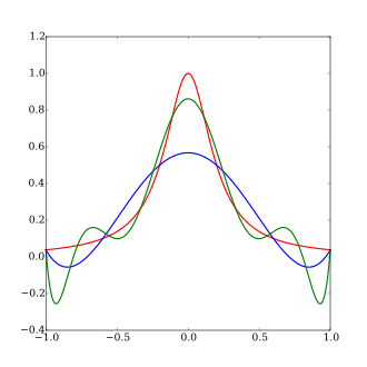
图源维基百科. 和数据无关.
The Chebyshev interpolation points
用这个方法解决采样位置不好导致的误差变大问题.
Theorem 4.3 The norm of the Lagrange interpolation operator has the value \(\lVert \boldsymbol{X} \rVert=\max _{a \leqslant x \leqslant b} \sum_{k=0}^n\left\lvert l_k(x)\right\rvert\) where the functions $\left\lbrace l_k ; k=0,1, \ldots, n\right\rbrace$ are defined by equation (4.3). Proof. The definition of a norm and equation (4.6) give the identity \(\begin{aligned} \lVert \boldsymbol{X} \rVert & =\sup _{\lVert f \rVert \leqslant 1}\lVert \boldsymbol{X}(f) \rVert \\ & =\sup _{\lVert f \rVert \leqslant 1} \max _{a \leqslant x \leqslant b}\left\lvert \sum_{k=0}^n f\left(x_k\right) l_k(x)\right\rvert \\ & =\max _{a \leqslant x \leqslant b} \sup _{\lVert f \rVert \leqslant 1} \left\lvert \sum_{k=0}^n f\left(x_k\right) l_k(x)\right\rvert \\ & =\max _{a \leqslant x \leqslant b} \sum_{k=0}^n\left\lvert l_k(x)\right\rvert \end{aligned}\) which is the required result.
解释解释每一个等号都是为什么:
The first quality: Consider the definition of norm of approximation operator: The norm of $X$ is written as $\lVert X \rVert$, and it is the smallest real number such that the inequality $\lVert \boldsymbol{X}(f) \rVert \leqslant\lVert \boldsymbol{X} \rVert\lVert f \rVert$ holds. Here, if $\lVert f \rVert$ is not equal to one, then suppose $\lVert f \rVert = a \neq 0$, Then
Left hand side: \(\begin{aligned} \lVert \boldsymbol{X}((1/a)f) \rVert &= \lVert (1/a)\boldsymbol{X}(f) \rVert \quad \text{the approximation operator of Lagrange interpolation is linear}\\ &= \lvert (1/a) \rvert\cdot \lVert \boldsymbol{X}(f) \rVert \quad \text{absolute homogeneity of norm} \end{aligned}\)
Right hand side: \(\lVert \boldsymbol{X} \rVert\lVert (1/a)f \rVert = \lvert (1/a) \rvert\cdot \lVert \boldsymbol{X} \rVert\lVert f \rVert\quad \text{absolute homogeneity of norm}\)
That is, $\lvert (1/a) \rvert$ appears on both the LHS and RHS of $\lVert \boldsymbol{X}(f) \rVert \leqslant\lVert \boldsymbol{X} \rVert\lVert f \rVert$ when $\lVert f \rVert \neq 1$, it can thus be cancelled out.
So \(\begin{aligned} \lVert \boldsymbol{X} \rVert &= \sup _{ \lVert f \rVert \neq 0} \frac{\lVert \boldsymbol{X}(f) \rVert }{\lVert f \rVert} \\ &= \sup _{\lVert f \rVert = 1} \frac{\lVert \boldsymbol{X}(f) \rVert }{\lVert f \rVert} \\ &= \sup _{\lVert f \rVert = 1} \lVert \boldsymbol{X}(f) \rVert \\ &= \sup _{\lVert f \rVert \leq 1} \lVert \boldsymbol{X}(f) \rVert \end{aligned}\) The second equality: this is by the definition of infinity norm.
The third equality:
Theorem (supremum of supremum is interchangeable) \(\sup _{a \in A} \sup _{b \in B} F(a, b)=\sup _{(a, b) \in A \times B} F(a, b)=\sup _{b \in B} \sup _{a \in A} F(a, b)\) Let us prove the first equality and the second follows symmetrically. Let $S_1=\sup _{a \in A} \sup _{b \in B} F(a, b)$ and $S_2=\sup _{(a, b) \in A \times B} F(a, b)$. Suppose that $S_1<S_2$. Then, since $S_2$ is the least upper bound of the set $\lbrace F(a, b):(a, b) \in A \times B\rbrace$, there exist $\left(a_0, b_0\right) \in A \times B$ with $S_1<F(a, b)$. But then \(F\left(a_0, b_0\right) \leq \sup _{b \in B} F\left(a_0, b\right) \leq \sup _{a \in A} \sup _{b \in B} F(a, b)=S_1\) a contradiction. Next, suppose that $S_2<S_1$. Then, because $S_1$ is the least upper bound of $\left\lbrace\sup _{b \in B} F(a, b): a \in A\right\rbrace$, it follows that there is some $a_0 \in A$ such that $S_2<\sup _{b \in B} F\left(a_0, b\right)$. Similarly, there now exists $b_0 \in B$ such that $S_2<F\left(a_0, b_0\right)$, a contradiction. $\square$
Here, $\left\lvert \sum_{k=0}^n f\left(x_k\right) l_k(x)\right\rvert$ is continuous and is defined on a closed interval, so $\max {a \leqslant x \leqslant b}\left\lvert \sum{k=0}^n f\left(x_k\right) l_k(x)\right\rvert = \sup {a \leqslant x \leqslant b}\left\lvert \sum{k=0}^n f\left(x_k\right) l_k(x)\right\rvert$.
Then \(\begin{aligned} &\sup _{\lVert f \rVert \leqslant 1} \max _{a \leqslant x \leqslant b}\left\lvert \sum_{k=0}^n f\left(x_k\right) l_k(x)\right\rvert \\ =&\sup _{\lVert f \rVert \leqslant 1} \sup _{a \leqslant x \leqslant b}\left\lvert \sum_{k=0}^n f\left(x_k\right) l_k(x)\right\rvert \\ =&\sup _{a \leqslant x \leqslant b} \sup _{\lVert f \rVert \leqslant 1} \left\lvert \sum_{k=0}^n f\left(x_k\right) l_k(x)\right\rvert \\ =&\max _{a \leqslant x \leqslant b} \sup _{\lVert f \rVert \leqslant 1} \left\lvert \sum_{k=0}^n f\left(x_k\right) l_k(x)\right\rvert \\ \end{aligned}\)
The fourth equality: when $f(x_k) = 1$ for all $k$, $\left\lvert \sum_{k=0}^n f\left(x_k\right) l_k(x)\right\rvert $ reaches its maximum. Since $\lVert f \rVert \leqslant 1$ is a closed constraint, this is also its supremum.
Recall that
Theorem 3.1 Let $\mathscr{A}$ be a finite-dimensional linear subspace of a normed linear space $\mathscr{B}$, and let $X$ be a linear operator from $\mathscr{B}$ to $\mathscr{A}$ that satisfies the projection condition (3.2). For any $f$ in $\mathscr{B}$, let $d^*$ be the least distance
\(d^*=\min _{a \in \mathbb{A}}\lVert f-a \rVert\) from $f$ to an element of $\mathscr{A}$. Then the error of the approximation $X(f)$ satisfies the bound
\[\lVert f-\boldsymbol{X}(f) \rVert \leqslant [1+\lVert \boldsymbol{X} \rVert] d^*\]
我们想知道 $\lVert \boldsymbol X \rVert$ 好不好,至少想知道他至少是多少. 上面他做了一些实验,我们可以用观测到的数据给出 $\lVert \boldsymbol X \rVert$ 的一个下界. \(\begin{aligned} \lVert \boldsymbol{X} \rVert &\geq \frac{\lVert f-\boldsymbol{X}(f) \rVert }{d^*} - 1 \\ & \geq \frac{\max \left\lvert f(x_i)-\boldsymbol{X}(f(x_i))\right\rvert}{d^{*+}} \\ & = (39.994889 / 0.015507)-1 =10 986.71 \end{aligned}\) 还是蛮大的,毕竟 $\boldsymbol X$ 只说了是从什么东西映射到了什么东西,没说采样的时候是怎样采样,所以可以相当大. 所以我们在采样的时候要选择比较安全的方式,比如使用 Chebyshev interpolation points.
但是要注意,Chebyshev interpolation points 并不是万金油,尽管使用了这种方法,误差也相当大的情况依然存在.