Fast Inverse Square Root

同时包含 Approximation theory and method ch11.

https://www.youtube.com/watch?v=p8u_k2LIZyo

Fast Inverse Square Root（快速倒数平方根）是一种算法，用于快速计算一个数的倒数平方根。该算法最早出现在Quake III Arena游戏引擎中，用于在计算机图形学中加速向量的归一化过程。

Fast Inverse Square Root算法的中文名称可以直译为”快速倒数平方根”。

今天看到一个很有意思的算法, 是关于快速计算 $1/\sqrt x $ 的. 很奇怪啊, 为什么会需要优化这个的计算呢?

```c float Q_rsqrt( float number ) { long i; float x2, y; const float threehalfs = 1.5F;

x2 = number * 0.5F;
y  = number;
i  = * ( long * ) &y;                       // evil floating point bit level hacking
i  = 0x5f3759df - ( i >> 1 );               // what the fuck? 
y  = * ( float * ) &i;
y  = y * ( threehalfs - ( x2 * y * y ) );   // 1st iteration //	y  = y * ( threehalfs - ( x2 * y * y ) );   // 2nd iteration, this can be removed

return y; } ```

https://en.wikipedia.org/wiki/Fast_inverse_square_root

在计算平面的法向量的时候, 我们需要把向量归一化, 也就是所谓的 normalize. 这样在我们计算向量乘法的时候, 假设我们现在有很多很多向量——就不会因为这些法向量的长度有大有小而带来误差.

具体一点的例子就如视频里面所说, 在计算一个多面物体被光源照射的时候, 反射强度就需要各个平面的法向量与光照向量点乘来计算反射强度.

我们考虑对一个float 类型的数做 fast inverse square root.

float 由 sign (1 bit), exponent (8 bit) 和 mantissa(23bit) 组成.

Sign 始终是 0 , 因为只有正数才能开方;
Exponent 记做 $\mathrm E$;
Mantissa 记做 $\mathrm M$;

float的值是:

\[\left(1+\frac{\mathrm{M}}{2^{23}}\right) \times 2^{\mathrm{E}-127}\]

这是比较数学的写法, 写得更好理解一点就是

\[\left(1+(\mathrm{M}>>23)\right) \times {(1 << (\mathrm{E}-127)})\]

或者

cpp (1 + (M >> 23)) << (E - 127)

就是M 右移 23 位, 加上 1 然后乘 Exponent. 乘一个 2 的指数相当于左移对应的位数.

我们先对 $\left(1+\frac{\mathrm{M}}{2^{23}}\right) \times 2^{\mathrm{E}-127}$ 取对数,

\[\log \left(1+\frac{\mathrm{M}}{2^{23}}\right) + \log 2^{\mathrm{E}-127} = \log \left(1+\frac{\mathrm{M}}{2^{23}}\right) + {\mathrm{E}-127}\]

在中学我们学过, $\ln x $ 在 $x = 1$ 附近可以用 $p(x) = x$ 来进行近似计算. 在这里我们需要用一个一次多项式来逼近 $\log _2(1+x)$ . $\frac{\mathrm{M}}{2^{23}}$ 是一个在 $[0,1]$ 里的数, 所以我们希望在区间 $[0,1]$ 里能达到最优近似.

以下提到的定理等等, 默认参考的是 Approximation Theory and Method, M. J. D. POWELL.

视频里给出的近似方式, 强制了 $x$ 的系数是 $1$:

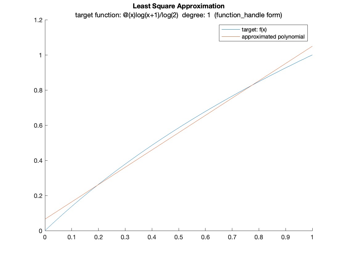
\[\log _2(1+\mathrm{x}) \approx \mathrm{x} + \mu\]

线说说不强制 $x$ 的系数的情况吧——用来逼近的集合是 $\mathscr A = \mathscr P_1$, 目标函数是 $f = \log _2(1+x)$, 也就是需要找到一组 $k, x$ 使得在区间 $[0,1]$ 上,

\[f = \log _2(1+x) \approx kx + \mu = p\]

使用 2-norm approximation, 我们希望

\[\arg_{k,\mu} \min\int_0 ^1 [f - p] \mathrm d x\] \[f = \log _2(1+x) \approx x + \mu = p\]

希望

\[\arg_{k,\mu} \min\int_0 ^1 [f - p] \mathrm d x\]

根据 least square approximation 的 characterization theorem, 我们希望

\[(e*, p) = 0,\quad \forall p \in \mathscr A\]

$e* = f - p ^* $ 是误差函数, $(\cdot , \cdot)$ 是函数的 inner product. 多说一点, 函数的 inner product 是这样定义的: 在区间 $[a,b]$ 上,

\[(f , g) = \int_a^b wfg \mathrm d x\]

其中 $w$ 是权重函数.

开始动手算, 我们希望误差对所有在 $\mathscr A $ 内的元素都有 0 内积. 对所有的元素有 0 内积, 实际上仅仅需要对 $\mathscr A$ 的一组基里面所有的元素有 0 内积就行了. 这里$\mathscr A \subset \mathscr P_2$, $\mathscr A$ 是一个线性空间, 所以对 $\mathscr A$ 里面所有的元素有 0 内积.

我们需要找一个 $\mathscr A$ 的基, 为了后续求解方程组方便, 我们最好找一组正交积. 在内积的定义是在区间 $[a, b]$ 上的定积分, 所以所有相关的函数都跟 $[a, b]$ 有关, 特别得在这里是 $[0,1]$. 记 $I= [a, b]$ . 我们可以用一套流程来生成多项式空间的正交基 (Theorem 11.3),

首先

\[\phi_0 = 1, x \in I\]

对于 $j \geqslant 0$, $\alpha_j$ 是这个:

\[\alpha_i=\left(\phi_i, x \phi_i\right) /\left\|\phi_j\right\|^2\]

然后得到 $\phi_1(x)$

\[\phi_1(x)=\left(x-\alpha_0\right) \phi_0(x), \quad a \leqslant x \leqslant b .\]

后面的流程都用不着了.

```matlab % least_square_approximation_syms.m

% define the function that we need to approximate syms x f = log(x + 1) / log(2); interval = [0, 1];

% the approximation set is of dimension (n + 1) % here it is family of polynomial of degree n n = 1;

phi0 = 1 + 0*x; alpha0 = dot_prod(phi0, x * phi0, interval) ./ norm_f(phi0, interval) .^ 2; phi1 = (x - alpha0) * phi0;

```

这样我们就得到了一组正交基.

```Matlab disp(“inner_product of the basis is:”) disp(dot_prod(phi0, phi1, interval)); disp(“phi0:”); disp(phi0); disp(“phi1:”); disp(phi1);

```

```matlab inner_product of the basis is: 0

phi0: 1

phi1: x - 1/2 ```

\[\phi_0 = 1; \quad \phi_1 = x - 1/2,\]

基记为 $B = \{ \phi_0, \phi_1\}.$

然后我们来找最优逼近 $p^$. 希望 $(p, e^) = 0, \forall p \in \mathscr A$ 也就是

\[(p, e^*) = 0, \forall p \in \mathscr A\]

也就是

\[(\phi_i, e^*) = 0, \quad i = 0, 1\]

展开 $e^*$:

\[(\phi_i, f - p^*) = 0, \quad i = 0, 1\]

移项,

\[(\phi_i, f) = (\phi_i, p^*) , \quad i = 0, 1\]

写成含 $\phi$ 的形式:

$(\phi_i, f)$ 是一个可以计算的确定的数, 右边的 $p^*$可以待定系数:

\[p^* = c_0 \phi_0 + c_1 \phi_1 = \sum_{i = ...} c_i \phi _i\] \[(\phi_i, f) = (\phi_i, c_0 \phi_0 + c_1 \phi_1), \quad i = 0, 1\]

右边展开,

\[(\phi_i, c_0 \phi_0 + c_1 \phi_1) = c_0 (\phi_i, \phi_0 ) +c_1(\phi_i, \phi_1), \quad i = 0, 1\]

因为是正交积, $\phi_i $ 在和不是自己内积的时候都变成 0:

\[(\phi_0, c_0 \phi_0 + c_1 \phi_1) = c_0 (\phi_0, \phi_0 ) \\ (\phi_1, c_0 \phi_0 + c_1 \phi_1) = c_1(\phi_1, \phi_1)\\\]

两个未知数, 两个方程, 实际上就是解一组线性方程组的问题:

\[(\phi_0, f) = c_0 (\phi_0, \phi_0 ) \\ (\phi_1, f) = c_1(\phi_1, \phi_1)\]

这样每个 $c_i$ 只需要计算一次除法就能得到.

\[c_0 = \frac{(\phi_0, f) }{\| \phi_0 \| ^ 2} \\ c_1 = \frac{(\phi_1, f) }{\| \phi_1 \| ^ 2} \\\]

拓展到 $i = 1, …, n$ 的时候,

\[(\phi_i, f) = \left(\phi_i, \sum_{j = 0}^{n} c_j \phi_j \right), \quad i = 0, ..., n\] \[(\phi_i, f) = \sum_{i = 0}^{n} c_j \left(\phi_i, \phi_j \right), \quad i = 0, ..., n\]

写得线性代数一点:

\[b = Ac\]

where

\[b_i =(\phi_i, f) , \\ A_{i,j} = \left(\phi_i, \phi_j \right), \\ c_j = c_j.\]

根据 characterization theorem, 线性方程组的解 $c$ 肯定是存在唯一的. 如果从矩阵 $A$ 的角度, …(待补充)

说回当前这个问题来, $f = \log _2(1+x)$,

用上面的结论我们可以算出:

matlab c0 = dot_prod(phi0, f, interval) / norm_f(phi0, interval) ^ 2; c1 = dot_prod(phi1, f, interval) / norm_f(phi1, interval) ^ 2; p_star = c0 * phi0 + c1 * phi1; disp(double(subs(p_star, x, 0))); disp(double(subs(p_star, x, 1) - subs(p_star, x, 0)));

```matlab 0.0652

0.9843 ```

为多项式系数, 所以 $p^* (x) = 0.9843x+ 0.0652$

approx_of_p2

但是这样后续处理的时候系数 $0.9843$ 就不是很方便,

那我们还是强制第一个系数是 1 看看.

我们希望

\[\arg_\mu \min \int _0^1 \left[ \log(x + 1) - (x + \mu)\right]^2 \mathrm dx\]

把这个问题转换成我们熟悉的问题:

\[\arg_\mu \min \int _0^1 \left[ \left( \log(x + 1) - x \right) - \mu)\right]^2 \mathrm dx\]

也就是目标函数是 $f = \left( \log(x + 1) - x \right)$, 希望用 $p \in \mathscr A = \mathscr P_0$ 逼近. 根据 characterization theorem, 我们希望 $\left(f - p^, 1 \right) = 0$ ($1$ 是 $\mathscr A$ 的基, $p^ = c_0 \cdot 1$).

$c_0$ 实际上就是 $\mu$ 了.

\[c_0 = (f, 1) /(1,1) =\int_0^1 f(x) \mathrm dx\]

mathematica f[x_] = Log[x + 1]/Log[2] - x; Integrate[f[x], {x, 0, 1}] N[%]

Output:

\[\frac{\log (8)-2}{\log (4)} \\ 0.057305\]

啊? 怎么和他们的 0.0430357 不一样?

好吧, 0.0430357 是用 uniform norm 或者叫 inf-norm 算的.

不过没关系, inf-norm 也好算. 这里斜率是固定的, 不需要用什么 exchange algorithm, 直接纯代数就能有一个 closed form.

关于 exchange algorithm, 详见____

跟刚才一样, 目标函数是 $f = \left( \log(x + 1) - x \right)$, 希望用 $p \in \mathscr A = \mathscr P_0$ 逼近. 根据 characterization theorem, 我们希望有 $n + 2 = 3$ 个点, 使得在三个点处误差函数 $e^* = f - p^*$ 符号交替得取到最大最小, 并且最大最小的绝对值一样. $f$ 的性质也蛮不错的, 在 0 和 1 处函数值都是 0. 所以 $\mu$ 就是 $f$ 在区间 $[0,1]$ 最大最小值的平均. 偷个懒, 用 Mathematica 算:

mathematica Maximize[{f[x], 0 <= x <= 1}, {x}]; x1 = N[%][[1]]; Minimize[{f[x], 0 <= x <= 1}, {x}]; x2 = N[%][[1]]; (x1 + x2) /2

Output:

mathematica 0.0430357

好了, 终于拿到了 0.0430357, 我们继续讨论最初的算法. 我们现在有

\[\log _2(1+\mathrm{x}) \approx \mathrm{x} + \mu\]

$\mu$ 是已知的, 并且我们不仅仅只有 inf-norm 下最优的 $\mu$ , 我们还有 2-norm 下最优的$\mu$ , 我们还有 $x$ 斜率不固定情况下的最优逼近.

\[\begin{align} &\log \left(\left(1+\frac{\mathrm{M}}{2^{23}}\right) \times 2^{\mathrm{E}-127}\right) \\ =& \log \left(1+\frac{\mathrm{M}}{2^{23}}\right) + {\mathrm{E}-127}\\ =&\frac{\mathrm{M}}{2^{23}} + \mu + {\mathrm{E}-127}\\ =&\frac{\mathrm{M}}{2^{23}} +\frac{2^{23}\mathrm{E}}{2^{23}} + \mu-127\\ =&\frac{\mathrm{M} + 2^{23}\mathrm{E}}{2^{23}} + \mu-127\\ \end{align}\]

待续.